
Introduction
Check the price of a flight today, then check it again tomorrow — you'll likely see a different number. That's not an accident. Airlines, ride-hailing platforms, and major e-commerce retailers have been running ML-powered pricing engines for years, adjusting prices in seconds based on demand signals, inventory levels, and competitor moves.
Most businesses, however, haven't caught up. They're still running rule-based systems or manual price tables built for stable market conditions — conditions that rarely exist in most industries today.
The cost of that gap is real. Static pricing leaves revenue on the table during demand spikes, fails to defend margins under competitive pressure, and can't respond to the kind of sudden market disruptions that have become routine.
This guide covers what it actually takes to get this right: the ML algorithms driving dynamic pricing, how to build a solid data foundation, a step-by-step implementation path, and the governance failures that have cost companies dearly when they skipped the controls.
Key Takeaways
- ML dynamic pricing adjusts prices in real time using demand signals, competitor data, customer behavior, and inventory — not fixed rules
- Gradient boosting models (XGBoost, LightGBM) are the most production-ready starting point; reinforcement learning is best for continuous optimization in complex environments
- Clean, multi-source data pipelines and pricing guardrails are prerequisites — not nice-to-haves
- Retail, transportation, energy, and insurance are actively deploying ML pricing with documented revenue impact
- Regulatory and ethical risks must be designed in from the start, not patched in later
Why ML Outperforms Traditional Dynamic Pricing Methods
Traditional pricing systems relied on analyst-built rule tables, ARIMA time-series models, and periodic A/B tests. These approaches assume relatively stable market conditions — and they fail badly when conditions shift fast.
Airline revenue management research documents exactly this failure mode: when demand shocks hit, historical databases update too slowly, and threshold-based alerts either miss the disruption or flood analysts with false positives. The system built for normal times becomes a liability in abnormal ones.
Three Concrete Advantages ML Brings
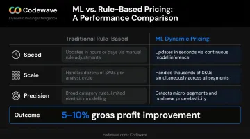
Speed: ML systems update prices in seconds. Manual or rule-based adjustments take hours or days — sometimes long enough for the market opportunity to disappear entirely.
Scale: A human analyst managing price tables can handle dozens of SKUs or segments. An ML model handles thousands simultaneously, with no degradation in decision quality.
Precision: ML identifies micro-segments and nonlinear price elasticity patterns that regression models and rule engines miss entirely. A customer who searched three times and abandoned their cart is not the same as a first-time visitor — and a well-trained model treats them differently.
The performance difference shows up in outcomes. BCG research on AI-powered retail pricing found gross profit improvements of 5%–10% from AI-driven pricing versus traditional approaches — though the actual uplift depends heavily on implementation quality and industry context.
What ML Dynamic Pricing Is Not
ML dynamic pricing is not a black box that sets prices without accountability. Specifically, it is not:
- Autonomous price-setting without human oversight
- Price gouging repackaged with better technology
- A one-time deployment that runs itself indefinitely
Every production-grade system requires ongoing governance, guardrails, and human review triggers — the sections below explain what that looks like in practice.
Key ML Algorithms Used in Dynamic Pricing
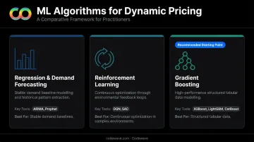
No single algorithm wins across all pricing contexts. The right choice depends on your data volume, environment complexity, and how much infrastructure you're willing to operate. Here's how the main options stack up.
Regression and Demand Forecasting Models
Regression models — linear, polynomial, ridge, and lasso — are typically the starting point. They model the relationship between price and demand using historical sales data, producing a demand curve that tells the pricing engine what happens to unit volume at each price point.
Layered on top, time-series models handle seasonality and cyclical patterns:
- ARIMA and Elastic-ARIMA for trend decomposition in stable demand environments
- Prophet for datasets with strong seasonal patterns and holiday effects
- Exponential smoothing for short-horizon forecasting where recent data should dominate
These models are interpretable, fast to train, and a practical baseline before moving to more complex approaches. Codewave uses XGBoost and Prophet across retail demand forecasting and pricing strategy engagements — making them a natural bridge into the gradient boosting methods covered below.
Reinforcement Learning for Continuous Optimization
Reinforcement learning (RL) is the most sophisticated approach. Instead of learning from labeled examples, the pricing model learns an optimal policy through trial and reward: set a price, observe the revenue outcome, update the policy accordingly.
Two algorithms dominate production pricing systems:
- Deep Q-Networks (DQN) work best for discrete price tiers — choosing between five predefined price levels for a product category, for example
- Soft Actor-Critic (SAC) handles continuous pricing environments where the model outputs any price within a range. It offers more stable convergence than earlier continuous-control methods
Alibaba's Tmall platform ran live field experiments using both: DQN for discrete price regions across 1,000 FMCG SKUs, and DDPG (a predecessor to SAC) for luxury items. The Tmall system was pre-trained on more than 40,000 SKUs and 2.4 million historical tuples before going live. That scale requirement defines RL's core constraint: without sufficient historical data and a simulation environment for pre-training, deploying directly in production carries real revenue risk.
Gradient Boosting and Ensemble Tree Models
For most teams building their first production pricing system, gradient boosting is the right starting point. XGBoost, LightGBM, and CatBoost handle mixed data types, missing values, and nonlinear feature interactions without requiring deep learning infrastructure.
They're particularly effective for competitor-based and inventory-sensitive pricing, ingesting structured tabular inputs:
- Competitor price feeds
- Current stock levels and stock-out risk scores
- Customer segment flags
- Day-of-week and time-to-event features
AWS's Adspert deployment documents production-grade Random Forest repricers. XGBoost appears in actuarial insurance pricing research and is part of Codewave's demand forecasting and pricing strategy work — which means the tooling, patterns, and failure modes are well understood before any client engagement starts.
Building the Data Foundation for Dynamic Pricing
Poor data is the most common reason pricing models underperform in production. A technically sophisticated model trained on incomplete or inconsistent data will produce confidently wrong price recommendations.
The Four Core Data Categories
Every ML dynamic pricing system needs inputs from four areas:
- Internal transactional data — historical sales volumes, prices paid, margins, and inventory levels. This is the baseline without which no model can estimate price elasticity
- Customer behavioral data — browsing patterns, purchase history, cart abandonment signals, and session frequency. These signals reveal willingness-to-pay at the individual or segment level
- External market data — competitor pricing feeds, macroeconomic indicators, and event or weather data where demand is sensitive to external factors
- Real-time streaming data — live inventory levels and active demand signals that trigger immediate price adjustments
Amazon's pricing operations ingest all four data types at scale. Profitero's research reported more than 2.5 million price changes per day on Amazon — though this figure comes from a third-party measurement and is not confirmed by Amazon directly. At that frequency, a data pipeline that lags by even minutes will push stale recommendations into live pricing decisions — a gap that compounds directly into margin loss.
Feature Engineering: Where Models Win or Lose
Feature selection is one of the top reasons pricing models fail in production. The most predictive features typically include:
- Price-to-competitor ratio (how your price compares to the nearest alternative)
- Stock-out risk score (probability of going out of stock within the forecast horizon)
- Time-to-event (for ticketing or perishable inventory)
- Customer segment label (high-intent vs. browsing, loyalty vs. new)
- Day-of-week and hour-of-day patterns
A model built on raw price and volume history alone will generalize poorly. The features above give the model context — without them, it can't distinguish a demand spike from a competitor stockout versus genuine willingness to pay more.
Data Quality Is Non-Negotiable
Missing historical data, inconsistent pricing records, and uncleaned competitor scrapes directly degrade model accuracy. There is no universal minimum data volume threshold, but Tmall's RL implementation relied on 2.4 million historical tuples as a case-specific baseline.
Minimum data requirements vary by modeling approach:
| Model Type | Recommended History | Notes |
|---|---|---|
| Gradient boosting | 12–18 months of transaction data | Requires consistent price and volume records throughout |
| Reinforcement learning | Higher volume required | Simulation environments often used to supplement real data during pre-training |
When historical data is sparse or inconsistent, synthetic data generation and pre-training on simulated environments can bridge the gap — but they introduce their own validation overhead that teams should plan for explicitly.
How to Implement ML-Based Dynamic Pricing: A Step-by-Step Guide
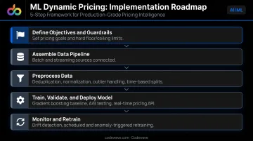
Step 1: Define Pricing Objectives and Guardrails
Before selecting any model, the business must decide what it's optimizing for:
- Revenue maximization — capture every dollar of willingness-to-pay
- Margin protection — defend profitability against competitive pressure
- Market share capture — price aggressively to grow volume
- Inventory clearance — move units before expiry or season end
These objectives lead to different reward functions and model architectures. Mixing them without clear priority creates models that optimize for nothing well.
Equally important: establish pricing floors and ceilings before deployment. Algorithms without hard limits can set prices that damage brand perception, trigger customer complaints, or violate regulatory requirements. Guardrails are not optional; treat them as part of the model specification itself.
Step 2: Assemble and Preprocess Your Data Pipeline
Build a pipeline that handles both batch and streaming sources:
- Batch: Historical sales data, CRM exports, product catalog
- Streaming: Live inventory signals, real-time competitor price feeds, active session data
Preprocessing steps before any model training:
- Deduplicate records and resolve conflicting price entries
- Normalize numerical features and encode categorical variables
- Handle outliers (promotional prices, data entry errors) that would distort elasticity estimates
- Apply time-based splits for validation — never random splits on time-series pricing data
At production scale, the volume demands are significant. FREE NOW's Kafka-based pricing pipeline handles approximately 200 million events daily, while Spresso's multi-armed bandit pricing system processes billions of impressions across thousands of SKUs. Tools like Apache Kafka, Snowflake, Apache Airflow, dbt, and Apache Flink represent the realistic infrastructure footprint for teams running ML pricing in production.
Step 3: Train, Validate, and Select Your Model
Use time-based train/validation/test splits, not random splits. Random splits allow look-ahead bias, where the model trains on future data and appears to perform well in testing but fails in production.
Evaluate models on pricing-relevant metrics, not just standard regression error:
- Simulated revenue uplift — would this model's recommendations have outperformed your baseline pricing?
- Price elasticity accuracy — does the model correctly predict demand response to price changes?
- RMSE on demand forecasts — a supporting metric, not the primary one
Start with gradient boosting (XGBoost or similar) as a reliable baseline. Move to RL-based approaches only after the baseline is performing well and you have the data volume and infrastructure to support it.
Step 4: Deploy Into a Real-Time Pricing Engine
Production deployment means the model outputs price recommendations through a pricing API that updates product listings, quote systems, or B2B pricing tables in near-real time. The API must handle latency requirements, since pricing decisions delayed by even a few seconds can miss the window they were optimized for.
Launch with A/B testing infrastructure. Compare ML pricing against your existing baseline before full rollout. Amazon's pricing experimentation research shows that random-days experimental designs can reduce standard errors in pricing tests by up to 60%. The experimental design matters as much as the model itself.
For teams moving from prototype to production, Codewave has built real-time pricing engines across retail, transportation, and fintech verticals using TensorFlow, Apache Kafka, Snowflake, XGBoost, and Kubernetes for model serving.
Step 5: Monitor, Govern, and Retrain
A deployed pricing model is not static. Two types of drift will degrade performance over time:
- Concept drift — the relationship between features and optimal price changes as market conditions evolve
- Data drift — the distribution of input data shifts (new competitor enters, consumer behavior changes)
Monitor these continuously. Tools like Evidently AI, Prometheus, and Grafana are designed for production ML monitoring and are part of Codewave's MLOps observability stack.
Establish retraining triggers:
- Scheduled retraining — weekly or monthly, regardless of detected drift
- Anomaly-driven retraining — triggered by sudden demand spikes, competitor pricing disruptions, or model performance drops below defined thresholds
Industry Applications: Where ML Dynamic Pricing Delivers Results
ML-driven pricing has moved well past proof-of-concept in several industries. Here's where it's producing measurable results.
E-Commerce and Retail
Catalog-scale, per-SKU price adjustments in real time are now table stakes for large retailers. Tmall's live field experiments with DQN and DDPG pricing demonstrated measurable revenue-conversion-rate improvements over control conditions — DQN reported an average DRCR of 5.10 versus 1.00 for the control group in daily-sales tests.
Transportation and Ride-Sharing
Uber and Lyft use RL-powered models that adjust pricing as demand shifts against driver supply. Uber's most significant change wasn't speed — it was structure. The company moved from multiplicative surge (surge multiplied base pay) to an additive mechanism: a fixed dollar amount added to base pay. Research shows this is more incentive-compatible for drivers and produces a stronger supply response.
Energy
Time-of-use electricity pricing is one of the oldest dynamic pricing models, and smart grid integration is making it more granular. Simulation research on PPO-based electricity dynamic pricing has reported 35% higher aggregator profit per sale versus A2C/DDPG alternatives — though large-scale live utility deployments remain limited.
Insurance
Progressive's Snapshot program personalizes renewal rates based on mileage, time of day, and hard braking data. By 2014, the program had collected over 10 billion miles of telematics data, representing $2 billion in written premium. The underlying algorithm isn't public, but Snapshot demonstrates what production-scale behavioral pricing looks like in practice.
Challenges and Ethical Considerations
Customer Trust and Transparency
Frequent or opaque price changes erode confidence. Customers who discover they paid more than a peer for the same product — based on browsing history or inferred demographics — respond badly. Clear communication about pricing logic, consistent behavior across sessions, and audits for discriminatory patterns are non-negotiable.
Regulatory Exposure
Dynamic pricing faces active regulatory scrutiny:
- The DOJ sued RealPage for an algorithmic pricing scheme in rental housing, alleging Sherman Act violations through landlord data-sharing used by pricing algorithms
- The FTC's 2025 surveillance pricing study identified personalized pricing based on location, browser history, and demographics as an area of active concern
- EU Directive 2019/2161 requires disclosure when prices are personalized using automated decision-making and individual profiling
Industries facing the highest scrutiny include housing, retail, and any sector where individual-level behavioral data drives pricing. In these environments, legal review before deployment belongs in the project plan alongside model development — not as a final checkpoint.

Model Governance Failures
Regulatory risk is external — model behavior is an internal threat you control directly. Unconstrained algorithms can drive prices up: two competing third-party Amazon seller algorithms drove a biology textbook to $23,698,655.93 through automated bidding. They can also race to the bottom in competitive markets, destroying margins for everyone. Pricing floors, ceilings, and human review triggers prevent both failure modes.
Frequently Asked Questions
What data do you need to build an ML-based dynamic pricing system?
You need four types: historical transaction data, customer behavioral signals, competitor pricing feeds, and real-time inventory or demand streams. Data quality matters as much as volume — inconsistent records or uncleaned competitor scrapes will degrade model accuracy regardless of the algorithm you choose.
Which machine learning algorithm is best for dynamic pricing?
There's no single best choice. Gradient boosting models (XGBoost, LightGBM) work well for structured tabular pricing data and are the most practical production starting point. Reinforcement learning is better suited for continuous optimization in complex, competitive environments, but it requires far more data and infrastructure. Start simpler and iterate.
How is dynamic pricing different from surge pricing?
Dynamic pricing continuously adjusts prices based on demand, competition, and inventory. Surge pricing is a reactive subset, triggered by sudden demand spikes (ride-hailing during bad weather is the classic example). All surge pricing is dynamic pricing, but not all dynamic pricing is surge pricing.
Can small or mid-sized businesses implement ML dynamic pricing?
Yes, with appropriate scope. SMBs can implement gradient boosting or demand-forecasting regression models without deep RL infrastructure or enterprise-scale compute. The key requirements are sufficient historical transaction data (at minimum 12–18 months of clean records) and a reliable data pipeline — not massive infrastructure budgets.
How do you prevent an ML pricing model from harming customer relationships?
Set hard floor and ceiling guardrails before deployment, and audit regularly for discriminatory patterns tied to inferred demographic signals. Run A/B tests before full rollout, and keep pricing communication transparent so customers aren't caught off guard by variability.
How long does it take to implement ML-based dynamic pricing?
A baseline gradient boosting model with existing clean data can reach production in 8–12 weeks. Full RL-based systems with real-time streaming pipelines typically require 4–6 months. Data readiness is almost always the biggest timeline driver — teams that underestimate data preparation time consistently miss their deployment targets.